PES-Learn Command-Line Interface (CLI) Tutorial#

PES-Learn is designed to work similarly to standard electronic structure theory packages: users can generate an input file with appropriate keywords, run the software, and get a result. This tutorial covers how to do exactly that. Here we generate a machine-learning model of the PES of water from start to finish (no knowledge of Python required!).

Generating Data#

Defining an internal coordinate grid#

Currently PES-Learn supports generating points across PESs by displacing in simple internal coordinates (a ‘Z-Matrix’). To do this, we must define a Z-Matrix in the input file. We first create an input file called input.dat:

vi input.dat

in the input file we define the Z-Matrix and the displacements:

O
H 1 r1
H 1 r2 2 a1

r1 = [0.85, 1.30, 10]
r2 = [0.85, 1.30, 10]
a1 = [90.0, 120.0, 10]

The syntax defining the internal coordinate ranges is of the form [start, stop, number of points], with the bounds included in the number of points. The angles and dihedrals are always specified in degrees. The units of length can be anything, though typically Angstrom or Bohr. Dummy atoms are supported (and in fact, are required if there are 3 or more co-linear atoms, otherwise in that case those internal coordinate configurations will just be deleted!). Labels for geometry parameters can be anything (RDUM, ROH1, A120, etc) as long as they do not start with a number. Parameters can be fixed with r1 = 1.0, etc. An equilibruim geometry can be specified in the order the internal coordinates appear with

eq_geom = [0.96,0.96,104.5]

and this will also be included.

Schemas and Templates#

Before we talk about building the rest of the input file by adding keywords that controll the program, lets first talk about schemas and template files. PES-Learn has two options to interface to the electronic structure theory program of choice. The first option is an interface to the QC program suite, namely QCEngine. QCEngine excecutes quantum chemistry programs with a standardized input and output system (QCSchema). With PES-Learn, all input specifications are written in the previously defined input file and PES-Learn will create simple python scripts that contain all the required information for QCEngine to pass to the quantum chemistry program.

That’s great but how do the specifications work? Let’s return to the input file that we defined in the last section and define some keywords to tell PES-Learn to create scripts to generate QCSchemas and run QCEngine. We will put these and any other keyword after the Z-Matrix and internal coordinate ranges:

...
schema_generate = true
schema_prog = psi4
schema_driver = energy
schema_method = ccsd(t)
schema_basis = cc-pvdz
schema_keywords = "{'reference: 'rhf'}"

The above keywords are all required for PES-Learn to utilize QCEngine/QCSchema.

schema_generate tells the program that you want to generate scripts to run QCEngine.
schema_prog tells what electronic structure theory program to use, QCEngine has a limited number of programs that it can interface to. Check the QCEngine Docs to see which programs are currently available.
schema_driver tells what kind of computation to run.
schema_method tells what level of theory to run the computations.
schema_basis tells the basis set to use for the computations.
schema_keywords tells QCEngine which program specific keywords to pass to the quantum chemistry program. These must be interpretable by the program you are using, and it is best practice to put them in quotes or PES-Learn may change the case.

For more information about these options and other schema related keywords, check out the Keywords section, all of the schema related keywords begin with schema_.

The advantage to interfacing with QCEngine is the ease of specifications to run computations, and the parsing that comes from the QCSchema outputs which is handled automatically by PES-Learn. When we run the code later on the auto-generated scripts to run QCEngine with geometries corresponding to the defined internal coordinate grid will be put into their own newly-created sub-directories like this:

PES_data/1/
PES_data/2/
PES_data/3/
...

With each numbered sub-directory in PES_data/ containing a different geometry. This PES_data folder can then be zipped up and sent to whatever computing resources you want to use.

Generating schemas is convenient, however, there are a limited number of programs that QCEngine interfaces to. If you want to use a program that is not in the list of programs interfacable to QCEngine, you can instead use a template input file. A template input file is a file named template.dat it is a cartesian coordinate input file for an electronic structure theory package such as Gaussian, Molpro, Psi4, CFOUR, QChem, NWChem, and so on. It does not matter what package you want to use, it only matters that the template.dat contains Cartesian coordinates, and computes an electronic energy by whatever means you wish. PES-Learn will use the template file to generate a bunch of (Guassian, Molpro, Psi4, etc) input files, each with different Cartesian geometries corresponding to the above internal coordinate grid. The template input file we will use in this example is a Psi4 input file which computes a CCSD(T)/cc-pvdz energy:

molecule h2o {
0 1
H 0.00 0.00 0.00
H 0.00 0.00 0.00
O 0.00 0.00 0.00
}

set {
reference rhf
basis cc-pvdz
}
energy('ccsd(t)')

The actual contents of the Cartesian coordinates does not matter. Later on when we run the code, the auto-generated input files with Cartesian geometries corresponding to our internal coordinate grid will be put into their own sub-directories similarly as above.

Data Generation Keywords#

Let’s go back to our PES-Learn input file, add a few keywords, and discuss them.

O
H 1 r1
H 1 r2 2 a1

r1 = [0.85, 1.30, 10]
r2 = [0.85, 1.30, 10]
a1 = [90.0, 120.0, 10]

...
# Data generation-relevant keywords
eq_geom = [0.96,0.96,104.5]
input_name = 'input.dat'
remove_redundancy = true
remember_redundancy = false
grid_reduction = 300

Comments (ignored text) can be specified with a # sign. All entries are case-insensitive. Multiple word phrases are seperated with an underscore. Text that doesn’t match any keywords is simply ignored (in this way, the use of comment lines is really not necessary unless your are commenting out keyword options). This means if you spell a keyword or its value incorrectly it will be ignored. The first occurance of a keyword will be used.

We discussed eq_geom before, it is a geometry forced into the dataset, and it would typically correspond to the global minimum at the level of theory you are using. It is often a good idea to create your dataset such that the minimum of the dataset is the true minimum of the surface, especially for vibrational levels applications.
input_name tells PES-Learn what to call the electronic structure theory input files (when using template files). ‘input.dat’` is the default value, no need to set it normally. Note that it is surrounded in quotes; this is so PES-Learn doesn’t touch it or change anything about it, such as lowering the case of all the letters.
remove_redundancy removes symmetry-redundant geometries from the internal coordinate grid. In this case, there is redundancy in the equivalent OH bonds and they will be removed.
remember_redundancy keeps a cache of redundant-geometry pairs, so that when the energies are parsed from the output files and the dataset is created later on, all of the original geometries are kept in the dataset, with duplicate energies for redundant geometries. If one does not use a permutation-invariant geometry for ML later, this may be useful.
grid_reduction reduces the grid size to the value entered. In this case it means only 300 geometries will be created. This is done by finding the Euclidean distances between all the points in the dataset, and extracting a maximally spaced ‘sub-grid’ of the size specified.

Running PES-Learn and generating data#

In the directory containing the PES-Learn input file input.dat (and template.dat if you so choose to use it), simply run

python path/to/PES-Learn/peslearn/driver.py

The code will then ask what you want to do, here we type g or generate and hit enter, and this is the output:

Do you want to 'generate' data, 'parse' data, or 'learn'? g

1000 internal coordinate displacements generated in 0.00741 seconds
Total displacements: 1001
Number of interatomic distances: 3
Geometry grid generated in 0.06 seconds
Removing symmetry-redundant geometries...  Redundancy removal took 0.01 seconds
Removed 450 redundant geometries from a set of 1001 geometries
Reducing size of configuration space from 551 datapoints to 300 datapoints
Configuration space reduction complete in 0.05 seconds
Your PES inputs are now generated. Run the jobs in the PES_data directory and then parse.
Data generation finished in 0.41 seconds
Total run time: 0.41 seconds

Now the python scripts (for schemas) or input files (for templates) with Cartesian coordinates corresponding to the internal coordinate grid are placed into a directory call PES_data with numbered sub-directories containing the unique coordinates.

Note

You do not have to use the command line to specify whether you want to generate, parse, or learn, you can instead specify the mode keyword in the input file:

mode = generate

This is at times convenient if computations are submitted remotely in an automated fashion, and the users are not directly interacting with a command line.

Now that we have built our inputs we are ready to run the computations!

If you are using schemas, then each of the numbered directories in PES_data will contain a python script that just needs to be excecuted. To do this in an automated fashion one might create a simple python script like the following

import os
os.chdir('PES_data')
for i in range(1,300):
    os.chdir(str(i))
    if "output.dat" not in os.listdir('.'):
        print(i, end=', ')
        os.system('python input.py')
    os.chdir('../')
os.chdir('../')
print('Your input scripts have been submitted.')

If you are working with this method and have compiled PES-Learn from source, make sure than you have QCEngine and QCSchema in your active environemnt, if you have installed PES-Learn from pip then it should have installed these dependencies already.

If you are instead working with templates, line 7 of this script can be changed to run your electronic sctructure program instead of Python. If using Psi4, for example, we can change line 7 to be

os.system('psi4 input.dat')

and then run your script. When your jobs have finished you are then able to move on to parsing the data.

Parsing output files#

Now that every Psi4 input file has been run, and there is a corresponding output.dat in each sub-directory of PES_data, we are ready to use PES-Learn to grab all of the energies, match them with the appropriate geometries, and create a dataset.

There are three schemes for parsing output files with PES-Learn * Automatic parsing from schemas * User-supplied Python regular expressions (regex) * cclib

Schemas are very useful and actually parse the data for us. The output is standardized, regardless of electronic structure program being utilized by QCEngine. The output is a JSON type strucure and the desired output (energy, gradient, Hessian, etc.) will be in the return_result object. PES-Learn is able to pull the result from this using regex.

Regular expressions are a pattern-matching syntax. Though they are somewhat tedious to use, they are completely general. Using the regular expression scheme requires

Inspecting the electronic structure theory software output file
Finding the line where the desired energy is
Writing a regular expression to match the line’s text and grab the desired energy.

cclib is a Python library of hard-coded parsing routines. It works in a lot of cases. At the time of writing, cclib supports parsing scfenergies, mpenergies, and ccenergies. These different modes attempt to find the highest level of theory SCF energy (Hartree-Fock or DFT), highest level of Moller-Plesset perturbation theory energy, or the highest level of theory coupled cluster energy. Since these are hard-coded routines that are version-dependent, there is no gurantee it will work! It is also a bit slower than regular expressions (i.e. milliseconds –> seconds slower)

Setting parsing keywords in the PES-Learn input file#

When using schemas, parsing the output files is as simple as adding a single keyword to our PES-Learn input.dat file.

# Parsing-relevent keywords
energy = schema

When you are parsing with regex or cclib, it is often a good idea to take a look at a successful output file in PES_data/. Here is the output file in PES_data/1/, which is the geometry corresponding to eq_geom that we defined earlier:

            **************************
            *                        *
            *        CCTRIPLES       *
            *                        *
            **************************


    Wave function   =    CCSD_T
    Reference wfn   =      RHF

    Nuclear Rep. energy (wfn)                =    9.168193296244223
    SCF energy          (wfn)                =  -76.026653661887252
    Reference energy    (file100)            =  -76.026653661887366
    CCSD energy         (file100)            =   -0.213480496782495
    Total CCSD energy   (file100)            =  -76.240134158669861

    Number of ijk index combinations:               35
    Memory available in words        :        65536000
    ~Words needed per explicit thread:            2048
    Number of threads for explicit ijk threading:    1

    MKL num_threads set to 1 for explicit threading.

    (T) energy                                =   -0.003068821713392
    * CCSD(T) total energy                  =  -76.243202980383259


    Psi4 stopped on: Thursday, 09 May 2019 01:51PM
    Psi4 wall time for execution: 0:00:01.05

*** Psi4 exiting successfully. Buy a developer a beer!

If we were to use cclib, we would put into our PES-Learn input.dat file:

# Parsing-relevant keywords
energy = cclib
energy_cclib = ccenergies

to grab coupled cluster energies. When using cclib, however, the CCSD energies might be grabbed instead of the CCSD(T) energies. It is always a good idea to check a few of your enegies after you parse, regardless of which method you are using.

Let’s not look at using Regular expressions (regex) to parse our outputs. One fact is always very important to keep in mind when using regular expressions in PES-Learn: PES-Learn always grabs the last matching entry in the output file.

This is good to know, since a pattern may match multiple entries in the output file, but it’s okay as long as you want the last one.

We observe that the energy we want is always contained in a line like

* CCSD(T) total energy                  =  -76.243202980383259

So the general pattern we want to match is total energy (whitespace) = (whitespace) (negative floating point number). We may put into our PES-Learn input file the following regular expression:

# Parsing-relevant keywords
energy = regex
energy_regex = 'total energy\s+=\s+(-\d+\.\d+)'

Here we have taken advantage of the fact that the pattern total energy does not appear anymore after the CCSD(T) energy in the output file. The above energy_regex line matches the words ‘total energy’ followed by one or more whitespaces \s+, an equal sign =, one or more whitespaces \s+, and then a negative floating point number -\d+\.\d+ which we have necessarily enclosed in parentheses to indicate that we only want to capture the number itself, not the whole line. This is a bit cumbersome to use, so if this in foreign to you I recommend trying out various regular expressions via trial and error using Regex101 or Pythex to ensure that the pattern is matched.

A few other valid energy_regex lines would be:

energy_regex = 'CCSD\(T\) total energy\s+=\s+(-\d+\.\d+)'

energy_regex = '=\s+(-\d+\.\d+)'

Note that above we had to “escape” the parentheses with backward slashes since it is a reserved character. If you want to be safe from parsing the wrong energy, more verbose is probably better.

Setting up the input file#

Here we have added out parsin keywords to out PES-Learn input file. (We could have had these keywords earlier as well, but to keep things simple I am only adding them when needed.)

O
H 1 r1
H 1 r2 2 a1

r1 = [0.85, 1.30, 10]
r2 = [0.85, 1.30, 10]
a1 = [90.0, 120.0, 10]

# Data generation-relevant keywords
eq_geom = [0.96,0.96,104.5]
input_name = 'input.dat'
remove_redundancy = true
remember_redundancy = false
grid_reduction = 300
schema_generate = true
schema_prog = psi4
schema_driver = energy
schema_method = ccsd(t)
schema_basis = cc-pvdz
schema_keywords = "{'reference: 'rhf'}"

# Parsing-relevant keywords
energy = schema
pes_name = 'PES.dat'      # name for the output file containing parsed data
sort_pes = true           # sort in terms of increasing energy
pes_format = interatomics # could also choose internal coordinates r1, r2, a1

Note that the example above is for parsing from schemas, and if you are parsing with cclib or regex, then you should include the appropriate energy, energy_cclib, and/or energy_regex keywords, instead of the schema keywords.

Parsing the output files and creating a dataset#

Just as before, we run PES-Learn

python path/to/PES-Learn/peslearn/driver.py

This time choose parse or p when prompted:

Do you want to 'generate' data, 'parse' data, or 'learn'? p
Parsed data has been written to PES.dat
Total run time: 0.38 seconds

This will compile all of the data necessary for generating machine learning models in the PES.dat file, which looks like this:

r0,r1,r2,E
518123981600,0.960000000000,0.960000000000,-76.243202980383
455484441900,0.950000000000,0.950000000000,-76.242743191056
494132369500,1.000000000000,0.950000000000,-76.242037809799
568831329800,1.000000000000,1.000000000000,-76.241196021922
494050142500,1.000000000000,1.000000000000,-76.240995054410
...

If you are working with schemas and one of the outputs failed (i.e. the QCSchema success entry is False) then PES-Learn will ommit this entry from your PES.dat file and write the failed directory number in a file errors.txt.

Creating Auto-Generated Machine Learning models of the PES#

Gaussian Process Regression#

We now have in our working directory a file called PES.dat, created with the routine above. An auto-optimized machine learning model of the surface can be produced by this dataset. Below we have added keywords to our PES-Learn input file which are relevant to training a ML model

O
H 1 r1
H 1 r2 2 a1

r1 = [0.85, 1.30, 10]
r2 = [0.85, 1.30, 10]
a1 = [90.0, 120.0, 10]

# Data generation-relevant keywords
eq_geom = [0.96,0.96,104.5]
input_name = 'input.dat'
remove_redundancy = true
remember_redundancy = false
grid_reduction = 300

# Parsing-relevant keywords
energy = regex
energy_regex = 'total energy\s+=\s+(-\d+\.\d+)'
pes_name = 'PES.dat'
sort_pes = true           # sort in terms of increasing energy
pes_format = interatomics # could also choose internal coordinates r1, r2, a1

# ML-relevant keywords
ml_model = gp              # Use Gaussian Process regression
pes_format = interatomics  # Geometry values in the PES file
use_pips = true            # Transform interatomic distances into permutation invariant polynomials
hp_maxit = 15              # Train 15 models with hyperparameter optimization, select the best
training_points = 200      # Train with 200 points (out of 300 total)
sampling = structure_based # Sample training set by maximizing Euclidean distances
n_low_energy_train = 1     # Force lowest energy point into training set

Note that a minimal working input file would only need the internal coordinate definition (because we are using PIPs and need to know the atom types!) and the ML relevant keywords:

O
H 1 r1
H 1 r2 2 a1

# ML-relevant keywords
ml_model = gp              # Use Gaussian Process regression
pes_format = interatomics  # Geometry values in the PES file
use_pips = true            # Transform interatomic distances into permutation invariant polynomials
hp_maxit = 15              # Train 15 models with hyperparameter optimization, select the best
training_points = 200      # Train with 200 points (out of 300 total)
sampling = structure_based # Sample training set by maximizing Euclidean distances
n_low_energy_train = 1     # Force lowest energy point into training set

running this input in the same way that we generated and parsed, now we select learn or l. This will try out several models and print the performance statistics in units of wavenumbers (cm \(^{-1}\))

Do you want to 'generate' data, 'parse' data, or 'learn'? l
Using permutation invariant polynomial transformation for molecule type  A2B
Beginning hyperparameter optimization...
Trying 15 combinations of hyperparameters
Training with 200 points (Full dataset contains 300 points).
Using structure_based training set point sampling.
Errors are root-mean-square error in wavenumbers (cm-1)
Hyperparameters:
{'morse_transform': {'morse': False}, 'pip': {'degree_reduction': False, 'pip': True}, 'scale_X': 'mm01', 'scale_y': None}
Test Dataset 5.38
Full Dataset 5.36
Median error: 4.18
Max 5 errors: [11.3 11.4 11.9 12.7 13.9]
Hyperparameters:
{'morse_transform': {'morse': True, 'morse_alpha': 2.0}, 'pip': {'degree_reduction': True, 'pip': True}, 'scale_X': 'mm11', 'scale_y': 'mm11'}
Test Dataset 0.94
Full Dataset 0.77
Median error: 0.53
Max 5 errors: [1.9 2.  2.  2.  2.2]
Hyperparameters:
{'morse_transform': {'morse': False}, 'pip': {'degree_reduction': True, 'pip': True}, 'scale_X': 'mm11', 'scale_y': 'mm11'}
Test Dataset 0.55
Full Dataset 0.51
Median error: 0.33
Max 5 errors: [1.2 1.3 1.3 1.5 1.8]
Hyperparameters:
{'morse_transform': {'morse': False}, 'pip': {'degree_reduction': False, 'pip': True}, 'scale_X': 'mm01', 'scale_y': 'std'}
Test Dataset 0.52
Full Dataset 0.42
Median error: 0.26
Max 5 errors: [1.1 1.1 1.1 1.2 1.2]
Hyperparameters:
{'morse_transform': {'morse': False}, 'pip': {'degree_reduction': False, 'pip': True}, 'scale_X': 'std', 'scale_y': None}
Test Dataset 5.38
Full Dataset 5.36
Median error: 4.17
Max 5 errors: [11.4 11.5 11.9 12.7 13.9]
Hyperparameters:
{'morse_transform': {'morse': False}, 'pip': {'degree_reduction': True, 'pip': True}, 'scale_X': 'std', 'scale_y': 'mm01'}
Test Dataset 0.86
Full Dataset 0.81
Median error: 0.52
Max 5 errors: [2.  2.  2.2 2.3 3. ]
Hyperparameters:
{'morse_transform': {'morse': False}, 'pip': {'degree_reduction': False, 'pip': True}, 'scale_X': 'mm11', 'scale_y': 'mm11'}
Test Dataset 0.54
Full Dataset 0.49
Median error: 0.35
Max 5 errors: [1.2 1.2 1.2 1.2 1.4]
Hyperparameters:
{'morse_transform': {'morse': True, 'morse_alpha': 1.2000000000000002}, 'pip': {'degree_reduction': True, 'pip': True}, 'scale_X': 'mm01', 'scale_y': None}
Test Dataset 9.84
Full Dataset 8.51
Median error: 6.29
Max 5 errors: [19.4 20.4 20.5 21.1 25.2]
Hyperparameters:
{'morse_transform': {'morse': True, 'morse_alpha': 1.8}, 'pip': {'degree_reduction': True, 'pip': True}, 'scale_X': None, 'scale_y': 'std'}
Test Dataset 0.28
Full Dataset 0.24
Median error: 0.15
Max 5 errors: [0.7 0.8 0.8 1.2 1.4]
Hyperparameters:
{'morse_transform': {'morse': False}, 'pip': {'degree_reduction': False, 'pip': True}, 'scale_X': None, 'scale_y': 'mm01'}
Test Dataset 0.91
Full Dataset 0.87
Median error: 0.57
Max 5 errors: [2.2 2.2 2.3 2.4 2.8]
Hyperparameters:
{'morse_transform': {'morse': False}, 'pip': {'degree_reduction': True, 'pip': True}, 'scale_X': None, 'scale_y': 'mm01'}
Test Dataset 0.97
Full Dataset 0.9
Median error: 0.61
Max 5 errors: [2.2 2.3 2.4 2.5 2.8]
Hyperparameters:
{'morse_transform': {'morse': False}, 'pip': {'degree_reduction': False, 'pip': True}, 'scale_X': 'mm11', 'scale_y': None}
Test Dataset 5.38
Full Dataset 5.37
Median error: 4.15
Max 5 errors: [11.4 11.5 12.  12.7 13.9]
Hyperparameters:
{'morse_transform': {'morse': True, 'morse_alpha': 1.3}, 'pip': {'degree_reduction': False, 'pip': True}, 'scale_X': 'mm01', 'scale_y': 'mm01'}
Test Dataset 1.37
Full Dataset 1.06
Median error: 0.57
Max 5 errors: [3.2 3.2 3.3 3.5 3.7]
Hyperparameters:
{'morse_transform': {'morse': False}, 'pip': {'degree_reduction': True, 'pip': True}, 'scale_X': 'mm11', 'scale_y': None}
Test Dataset 5.7
Full Dataset 5.68
Median error: 4.33
Max 5 errors: [13.  13.8 14.7 14.7 15.1]
Hyperparameters:
{'morse_transform': {'morse': True, 'morse_alpha': 1.5}, 'pip': {'degree_reduction': True, 'pip': True}, 'scale_X': 'mm01', 'scale_y': 'mm01'}
Test Dataset 1.3
Full Dataset 1.03
Median error: 0.65
Max 5 errors: [2.9 2.9 3.  3.  3.1]

###################################################
#                                                 #
#     Hyperparameter Optimization Complete!!!     #
#                                                 #
###################################################

Best performing hyperparameters are:
[('morse_transform', {'morse': True, 'morse_alpha': 1.8}), ('pip', {'degree_reduction': True, 'pip': True}), ('scale_X', None), ('scale_y', 'std')]
Fine-tuning final model architecture...
Hyperparameters:  {'morse_transform': {'morse': True, 'morse_alpha': 1.8}, 'pip': {'degree_reduction': True, 'pip': True}, 'scale_X': None, 'scale_y': 'std'}
Final model performance (cm-1):
Test Dataset 0.28  Full Dataset 0.24     Median error: 0.15  Max 5 errors: [0.7 0.8 0.8 1.2 1.4]

Saving ML model data...
Total run time: 66.25 seconds

Training with just 200 points, the best model had a RMSE on the 100-point test set of 0.28 cm \(^{-1}\), and the full 300 point dataset had a RMSE of 0.24 cm \(^{-1}\). This is absurdly accurate; it’s a good thing we used grid_reduction back when generating our data to reduce our dataset from 551 points to just 300! We clearly did not need more than a few hundred points to model this portion of the PES of water; any more computations would have been unnecessary! This is why it is important to probe how much data one needs along the surface at a meaningful but low level of theory.

Using the GP Model#

After running the above, PES-Learn creates a directory called model1data (subsequently trained models will not overwrite this, but instead create new directories model2data, model3data, etc.). Inside this directory is a variety of files which are self-explanatory.

The most important file is the auto-generated Python script compute_energy.py which can be used to evaluate new energies using the model. It needs to be in the same directory as PES.dat and model.json to work. It contains a function pes() which takes one or more cartesian or internal coordinate arguments and outputs one or more energies corresponding to the geometries. If the argument cartesian=False is set, you must supply coordinates in the exact same format and exact same order as the model was trained on (i.e. the format in PES.dat). If the argument cartesian=True is set, cartesian coordinates are supplied in the same order as given in a typical PES_data input file (not the template.dat file). Cartesians can only be supplied if the model was trained on interatomic distances or PIPs of the interatomic distances.

The compute_energy.py file can be imported and used. Here’s an example python script use_model.py which imports the pes function and evaluates some energies at some cartesian geometries.

from compute_energy import pes

cart_geoms = [[0.0000000000, 0.0000000000, 1.1000000000, 0.0000000000, 0.7361215932, -0.4250000000, 0.0000000000, 0.0000000000, 0.0000000000],
            [0.0000000000, 0.2000000000, 1.2000000000, 0.0000000000, 0.7461215932, -0.4150000000, 0.0000000000, 0.0000000000, 0.1000000000],
            [0.0000000000, 0.1000000000, 1.3000000000, 0.0000000000, 0.7561215932, -0.4350000000, 0.0000000000, 0.0000000000, 0.2000000000]]

energies1 = pes(cart_geoms)
print(energies1)

interatomic_geoms = [[1.494050142500,1.000000000000,1.000000000000],
                    [1.597603916000,1.000000000000,0.950000000000],
                    [1.418793563200,1.000000000000,0.950000000000]]

energies2 = pes(interatomic_geoms, cartesian=False)
print(energies2)

The print statements yield the following output. The energies are in units of Hartrees (which are the unit of energy in our PES.dat which the model was trained on).

[[-76.20462724]
[-76.21835841]
[-76.21467994]]
[[-76.24099496]
[-76.24031118]
[-76.24024971]]

Note

Just as in the above example, it is possible to feed in multiple geometric parameters into the pes() function. If you have multiple geometries that you would like to feed into this function, it is much more efficient to feed them all into the function at once, rather than in some loop feeding them in one at a time.

Neural Network Regression#

Neural networks (NNs) are recommended for training sets of size 1000 and above for efficiency. This is because the hyperparameter tuning of NNs takes much longer than GPs, so there is an initial up-front cost to training NNs that GPs do not have. The NN building code can be broken down into three steps:

Neural architecture search (NAS)
Hyperparameter tuning
Learning rate optimization

Early stopping is used more aggressively in the first steps than in the last. Therefore, the performance of models during the NAS and hyperparameter tuning steps should not be taken as final; the training of the models is being stopped early to save time.

Batch learning with the L-BFGS optimizer is currently the only option. For high-level regression tasks, it is far superior to 1st order optimizers such as Adam, SGD, and RMSProp.

The Neural Architecture Search (NAS) tries out several hidden layer structures. One can override default NAS hidden layer strucutres with the keyword nas_trial_layers with the syntax nas_trial_layers = [[32], [32,32], [256]], which would try out NNs with a single hidden layer of 32 nodes, two hidden layers with 32 nodes, and a single hidden layer with 256 nodes. The default NAS space is very large, so if you observe on your first run with the default NAS space that your dataset does better with a large number of nodes ([256,256] for example) you may consider restricting the NAS space on future runs using the nas_trial_layers keyword. There should be at least 3 hidden layer structures in the NAS space.

Hyperparameter tuning is similar to the GP model optimizer. The learning rate optimizer is self-explanatory. There are checks in place to detect performance plateaus (in which learning rate decay triggers), or overfitting (in which case training is halted).

For neural networks, a validation set must be specified since they are more prone to overfitting. The validation points are sampled from all points which are not training set points. If one does not specify a number of validation points, by default half of the test set points are converted to validation set points. If you dataset has 1000 points and 800 are used for training, there would by default be 100 validation points and 100 test points. The validation error is used to optimize hyperparameters, while the test set error is not used for anything, though it is printed in all cases.

A neural network can be trained with minimal modification of the GP input used previously:

O
H 1 r1
H 1 r2 2 a1

# ML-relevant keywords
ml_model = nn              # Use Neural Network regression
pes_format = interatomics  # Geometry values in the PES file
use_pips = true            # Transform interatomic distances into permutation invariant polynomials
hp_maxit = 15              # Train 15 models with hyperparameter optimization, select the best
training_points = 200      # Train with 200 points (out of 300 total)
validation_points = 50     # Validate with  50 points (50 left over for testing)
sampling = structure_based # Sample training set by maximizing Euclidean distances
n_low_energy_train = 1     # Force lowest energy point into training set
nas_trial_layers = [[32], [32,32], [64], [16,16,16]] # NAS hidden layer trial structures

The output from running PES-Learn gives:

Do you want to 'generate' data, 'parse' data, or 'learn'? l
Using permutation invariant polynomial transformation for molecule type  A2B
Number of validation points not specified. Splitting test set in half --> 50% test, 50% validation
Training with 200 points. Validating with 50 points. Full dataset contains 300 points.
Using structure_based training set point sampling.
Errors are root-mean-square error in wavenumbers (cm-1)

Performing neural architecture search...

Hidden layer structure:  [32]
Hyperparameters:  {'morse_transform': {'morse': False}, 'scale_X': {'scale_X': 'std', 'activation': 'tanh'}, 'scale_y': 'std', 'pip': {'degree_reduction': False, 'pip': True}, 'layers': [32]}
Test set RMSE (cm-1):  5.11  Validation set RMSE (cm-1):  5.03 Full dataset RMSE (cm-1):  4.40
Hidden layer structure:  [64]
Hyperparameters:  {'morse_transform': {'morse': False}, 'scale_X': {'scale_X': 'std', 'activation': 'tanh'}, 'scale_y': 'std', 'pip': {'degree_reduction': False, 'pip': True}, 'layers': [64]}
Test set RMSE (cm-1):  6.30  Validation set RMSE (cm-1):  4.59 Full dataset RMSE (cm-1):  5.06
Hidden layer structure:  [16, 16, 16]
Hyperparameters:  {'morse_transform': {'morse': False}, 'scale_X': {'scale_X': 'std', 'activation': 'tanh'}, 'scale_y': 'std', 'pip': {'degree_reduction': False, 'pip': True}, 'layers': [16, 16, 16]}
Test set RMSE (cm-1):  5.83  Validation set RMSE (cm-1):  6.52 Full dataset RMSE (cm-1):  4.99
Hidden layer structure:  [32, 32]
Hyperparameters:  {'morse_transform': {'morse': False}, 'scale_X': {'scale_X': 'std', 'activation': 'tanh'}, 'scale_y': 'std', 'pip': {'degree_reduction': False, 'pip': True}, 'layers': [32, 32]}
Test set RMSE (cm-1):  1.67  Validation set RMSE (cm-1):  1.69 Full dataset RMSE (cm-1):  1.57

Neural architecture search complete. Best hidden layer structures: [[32, 32], [32], [16, 16, 16]]

Beginning hyperparameter optimization...
Trying 15 combinations of hyperparameters
Hyperparameters:
{'layers': (32,), 'morse_transform': {'morse': True, 'morse_alpha': 1.6}, 'pip': {'degree_reduction': False, 'pip': True}, 'scale_X': {'activation': 'tanh', 'scale_X': 'std'}, 'scale_y': 'mm11'}
Test set RMSE (cm-1):  2.98  Validation set RMSE (cm-1):  2.67 Full dataset RMSE (cm-1):  2.94
Hyperparameters:
{'layers': (32,), 'morse_transform': {'morse': False}, 'pip': {'degree_reduction': False, 'pip': True}, 'scale_X': {'activation': 'tanh', 'scale_X': 'mm11'}, 'scale_y': 'mm01'}
Test set RMSE (cm-1): 17.35  Validation set RMSE (cm-1): 16.15 Full dataset RMSE (cm-1): 17.24
Hyperparameters:
{'layers': (32, 32), 'morse_transform': {'morse': True, 'morse_alpha': 1.6}, 'pip': {'degree_reduction': False, 'pip': True}, 'scale_X': {'activation': 'tanh', 'scale_X': 'mm11'}, 'scale_y': 'mm01'}
Test set RMSE (cm-1):   inf  Validation set RMSE (cm-1):   inf Full dataset RMSE (cm-1):   inf
Hyperparameters:
{'layers': (16, 16, 16), 'morse_transform': {'morse': True, 'morse_alpha': 1.9000000000000001}, 'pip': {'degree_reduction': True, 'pip': True}, 'scale_X': {'activation': 'tanh', 'scale_X': 'std'}, 'scale_y': 'std'}
Test set RMSE (cm-1):  4.13  Validation set RMSE (cm-1):  4.00 Full dataset RMSE (cm-1):  3.65
Hyperparameters:
{'layers': (32,), 'morse_transform': {'morse': False}, 'pip': {'degree_reduction': True, 'pip': True}, 'scale_X': {'activation': 'tanh', 'scale_X': 'mm11'}, 'scale_y': 'std'}
Test set RMSE (cm-1):  1.49  Validation set RMSE (cm-1):  1.42 Full dataset RMSE (cm-1):  1.31
Hyperparameters:
{'layers': (32, 32), 'morse_transform': {'morse': True, 'morse_alpha': 1.6}, 'pip': {'degree_reduction': False, 'pip': True}, 'scale_X': {'activation': 'tanh', 'scale_X': 'mm11'}, 'scale_y': 'std'}
Test set RMSE (cm-1):   inf  Validation set RMSE (cm-1):   inf Full dataset RMSE (cm-1):   inf
Hyperparameters:
{'layers': (32,), 'morse_transform': {'morse': False}, 'pip': {'degree_reduction': False, 'pip': True}, 'scale_X': {'activation': 'tanh', 'scale_X': 'std'}, 'scale_y': 'mm11'}
Test set RMSE (cm-1): 25623.45  Validation set RMSE (cm-1): 44170.74 Full dataset RMSE (cm-1): 20903.16
Hyperparameters:
{'layers': (16, 16, 16), 'morse_transform': {'morse': False}, 'pip': {'degree_reduction': True, 'pip': True}, 'scale_X': {'activation': 'tanh', 'scale_X': 'std'}, 'scale_y': 'mm11'}
Test set RMSE (cm-1):  4.87  Validation set RMSE (cm-1):  3.20 Full dataset RMSE (cm-1):  3.10
Hyperparameters:
{'layers': (32, 32), 'morse_transform': {'morse': False}, 'pip': {'degree_reduction': True, 'pip': True}, 'scale_X': {'activation': 'tanh', 'scale_X': 'std'}, 'scale_y': 'std'}
Test set RMSE (cm-1):  0.81  Validation set RMSE (cm-1):  0.82 Full dataset RMSE (cm-1):  0.71
Hyperparameters:
{'layers': (16, 16, 16), 'morse_transform': {'morse': False}, 'pip': {'degree_reduction': True, 'pip': True}, 'scale_X': {'activation': 'tanh', 'scale_X': 'mm11'}, 'scale_y': 'std'}
Test set RMSE (cm-1):  2.61  Validation set RMSE (cm-1):  2.43 Full dataset RMSE (cm-1):  2.11
Hyperparameters:
{'layers': (32, 32), 'morse_transform': {'morse': True, 'morse_alpha': 1.5}, 'pip': {'degree_reduction': False, 'pip': True}, 'scale_X': {'activation': 'tanh', 'scale_X': 'mm11'}, 'scale_y': 'std'}
Test set RMSE (cm-1):  4.09  Validation set RMSE (cm-1):  3.02 Full dataset RMSE (cm-1):  3.41
Hyperparameters:
{'layers': (32,), 'morse_transform': {'morse': True, 'morse_alpha': 1.8}, 'pip': {'degree_reduction': True, 'pip': True}, 'scale_X': {'activation': 'tanh', 'scale_X': 'mm11'}, 'scale_y': 'mm11'}
Test set RMSE (cm-1):  1.99  Validation set RMSE (cm-1):  1.93 Full dataset RMSE (cm-1):  2.23
Hyperparameters:
{'layers': (16, 16, 16), 'morse_transform': {'morse': False}, 'pip': {'degree_reduction': False, 'pip': True}, 'scale_X': {'activation': 'tanh', 'scale_X': 'std'}, 'scale_y': 'mm01'}
Test set RMSE (cm-1):   inf  Validation set RMSE (cm-1):   inf Full dataset RMSE (cm-1):   inf
Hyperparameters:
{'layers': (16, 16, 16), 'morse_transform': {'morse': False}, 'pip': {'degree_reduction': False, 'pip': True}, 'scale_X': {'activation': 'tanh', 'scale_X': 'std'}, 'scale_y': 'std'}
Test set RMSE (cm-1):  5.83  Validation set RMSE (cm-1):  6.52 Full dataset RMSE (cm-1):  4.99
Hyperparameters:
{'layers': (16, 16, 16), 'morse_transform': {'morse': True, 'morse_alpha': 1.6}, 'pip': {'degree_reduction': True, 'pip': True}, 'scale_X': {'activation': 'tanh', 'scale_X': 'std'}, 'scale_y': 'mm11'}
Test set RMSE (cm-1):  2.82  Validation set RMSE (cm-1):  2.70 Full dataset RMSE (cm-1):  2.61

###################################################
#                                                 #
#     Hyperparameter Optimization Complete!!!     #
#                                                 #
###################################################

Best performing hyperparameters are:
[('layers', (32, 32)), ('morse_transform', {'morse': False}), ('pip', {'degree_reduction': True, 'pip': True}), ('scale_X', {'activation': 'tanh', 'scale_X': 'std'}), ('scale_y', 'std')]
Optimizing learning rate...
Hyperparameters:  {'layers': (32, 32), 'morse_transform': {'morse': False}, 'pip': {'degree_reduction': True, 'pip': True}, 'scale_X': {'activation': 'tanh', 'scale_X': 'std'}, 'scale_y': 'std', 'lr': 1.0}
Test set RMSE (cm-1): 316275944698408704.00  Validation set RMSE (cm-1): 278706602952744288.00 Full dataset RMSE (cm-1): 269540779801922272.00
Hyperparameters:  {'layers': (32, 32), 'morse_transform': {'morse': False}, 'pip': {'degree_reduction': True, 'pip': True}, 'scale_X': {'activation': 'tanh', 'scale_X': 'std'}, 'scale_y': 'std', 'lr': 0.8}
Test set RMSE (cm-1):  5.71  Validation set RMSE (cm-1):  4.43 Full dataset RMSE (cm-1):  3.70
Hyperparameters:  {'layers': (32, 32), 'morse_transform': {'morse': False}, 'pip': {'degree_reduction': True, 'pip': True}, 'scale_X': {'activation': 'tanh', 'scale_X': 'std'}, 'scale_y': 'std', 'lr': 0.6}
Test set RMSE (cm-1): 42.92  Validation set RMSE (cm-1): 27.75 Full dataset RMSE (cm-1): 21.25
Hyperparameters:  {'layers': (32, 32), 'morse_transform': {'morse': False}, 'pip': {'degree_reduction': True, 'pip': True}, 'scale_X': {'activation': 'tanh', 'scale_X': 'std'}, 'scale_y': 'std', 'lr': 0.5}
Test set RMSE (cm-1):  0.81  Validation set RMSE (cm-1):  0.82 Full dataset RMSE (cm-1):  0.71
Hyperparameters:  {'layers': (32, 32), 'morse_transform': {'morse': False}, 'pip': {'degree_reduction': True, 'pip': True}, 'scale_X': {'activation': 'tanh', 'scale_X': 'std'}, 'scale_y': 'std', 'lr': 0.4}
Test set RMSE (cm-1):  1.30  Validation set RMSE (cm-1):  0.98 Full dataset RMSE (cm-1):  1.06
Hyperparameters:  {'layers': (32, 32), 'morse_transform': {'morse': False}, 'pip': {'degree_reduction': True, 'pip': True}, 'scale_X': {'activation': 'tanh', 'scale_X': 'std'}, 'scale_y': 'std', 'lr': 0.2}
Test set RMSE (cm-1):  1.50  Validation set RMSE (cm-1):  1.12 Full dataset RMSE (cm-1):  1.19
Fine-tuning final model...
Hyperparameters:  {'layers': (32, 32), 'morse_transform': {'morse': False}, 'pip': {'degree_reduction': True, 'pip': True}, 'scale_X': {'activation': 'tanh', 'scale_X': 'std'}, 'scale_y': 'std', 'lr': 0.5}
Epoch 1 Validation RMSE (cm-1): 2008.26
Epoch 2 Validation RMSE (cm-1): 719.83
Epoch 3 Validation RMSE (cm-1): 411.05
...
Epoch 355 Validation RMSE (cm-1):  0.95
Test set RMSE (cm-1):  1.04  Validation set RMSE (cm-1):  0.95 Full dataset RMSE (cm-1):  0.80
Model optimization complete. Saving final model...
Saving ML model data...
Total run time: 957.76 seconds

The final results is a Test/Validation/Full dataset RMSE (cm-1) of 1.04, 0.95, and 0.80, respectively. Not quite as good as the GP models, but still about as accurate as you would ever want it to be!

Using the NN model#

The neural networks can be used in the exact same way as the GP models outlined above. The trained model is easily accessible using the compute_energy.py file. Model performance and the datasets are also saved.

Kernel Ridge Regression#

Kernel ridge regression (KRR) models have the advantage that they are typically pretty quick to train, even though the hyperparameter space is considerably larger than the GP or NN space. The disadvantage compared to GP and NN models is that the KRR models are typically less accurate when generated completely automatically.

The automated default procedure for KRR models is over a large space, however if a user notices that a particular type of model is better than others, the ability to reduce the hyperparameter space is available.

To run the default KRR hyperparameter optimization scheme, we can slightly modify the GP or NN schemes from above:

O
H 1 r1
H 1 r2 2 a1

# ML-relevant keywords
ml_model = krr             # Use Kernel Ridge Regression
kernel = verbose           # Use all types of available kernels in hyperparameter optimization
pes_format = interatomics  # Geometry values in the PES file
use_pips = true            # Transform interatomic distances into permutation invariant polynomials
hp_maxit = 200             # Train 15 models with hyperparameter optimization, select the best
training_points = 200      # Train with 200 points (out of 300 total)
sampling = structure_based # Sample training set by maximizing Euclidean distances
n_low_energy_train = 1     # Force lowest energy point into training set

Here we set the ml_model keyword to krr and the kernel = verbose option was added. kernel = verbose tells PES-Learn to use every type of available kernel for hyperparameter optimization. This does include quite a few options so it might be good to start with this option and then look at the results and see which kernels work best and then narrow your search. Alternatively you could increase the number of hyperparameter optimizations with hp_maxit. Note that the extent of the hyperparameter space for KRR gives over 100,000 possibilities with the kernel keyword set to verbose!

This can be excecuted in the same way as the GP or NN models and gives similar output which has been ommited here to reduce space. The main difference is the added R \(^2\) calculation that gets printed with each hyperparameter optimization.

If you find a kernel that works well and you want to reduce the hyperparameter space to optimize over, you can modify the kernel keyword to be precomputed and add an additional keyword precomputed_kernel =. For more information about using precomputed kernels, check out the KRR Examples page (link to be added).

Using the KRR model#

The neural networks can be used in the exact same way as the GP or NN models outlined above. The trained model is easily accessible using the compute_energy.py file. Model performance and the datasets are also saved.

Analyzing model performance using Python#

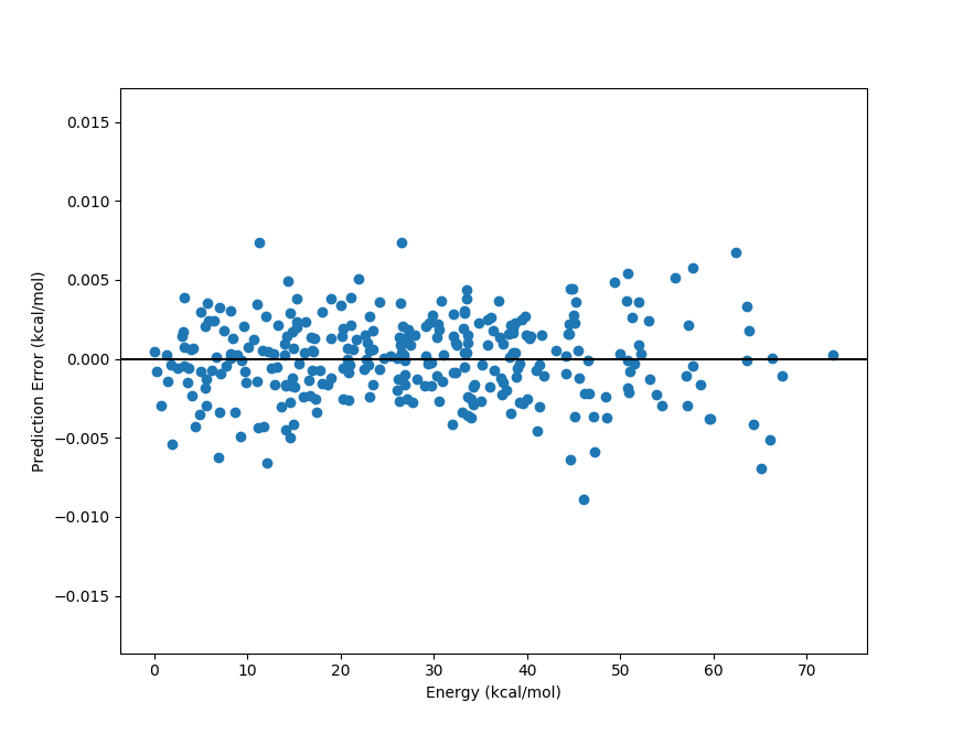
One can use Python to further analyze the performance of a PES-Learn ML model. Here’s a simple example of how to evaluate the error of a PES-Learn ML model as a function of energy relative to the global minimum. The following python file analyze.py must be in the same directory as the auto-generated compute_energy.py file, the dataset file PES.dat, and the saved ML model file model.json, model.pt, or model.joblib depending on the type of ML method used to build the model.

from compute_energy import pes
import pandas as pd

# load data
full_dataset = pd.read_csv('PES.dat')
# Split data into column arrays of geometries and energies
geoms = full_dataset.values[:, :-1]
energies = full_dataset.values[:, -1].reshape(-1,1)

# Geometries are ready to be sent through the model
predicted_energies = pes(geoms, cartesian=False)

# Prepare a plot of energy vs prediction error
relative_energies = (energies - energies.min())
errors = predicted_energies - energies


# Plot error distribution
import matplotlib.pyplot as plt
relative_energies *= 627.509 # convert to kcal/mol
errors *= 627.509
plt.scatter(relative_energies, errors)
plt.axhline(color='black')
plt.xlabel('Energy (kcal/mol)')
plt.ylabel('Prediction Error (kcal/mol)')
plt.show()